Image Classification

Papers:

• ImageNet Classification with Deep Convolutional Neural Networks by Krizhevsky, et al [AlexNet]
• Very Deep Convolutional Networks for Large Scale Image Recognition by Simonyan, et al [VGG]
• Going Deeper with Convolutions by Szegedy, et al [GoogLeNet]

• At the time, object recognition was machine learning based, with relatively smaller image datasets (like CIFAR)
• This paper came about after the creation of larger, more granular datasets like ImageNet and LabelMe
• CNN's were employed in order to learn features from 1000s of types of objects, for millions of images

• It's worth noting that CNN's have far fewer connections and parameters to standard NNs, so they are easier to train with only a slightly worse theoretical best performance
• This paper proposes an implementation of (for the time) an extremely large CNN, powered by GPU parallelization and a highly optimised version of 2D convolution

• Trained one of the largest convolutional neural networks to date on the subsets of ImageNet used in the ILSVRC-2010 and ILSVRC-2012 competitions
• Achieved the best results on these datasets
• Created and released GPU optimised versions of operations like 2D convolutions
• Tackled overfitting (created by the size of the network) via several effective techniques

• ImageNet consists of variable-resolution images, while the CNN requires a constant input dimensionality.
• The images were hence downsampled to 256x256. Given a rectangular image, the image was first rescaled such that the shorter side was of length 256, and then the central 256x256 patch was cropped out.

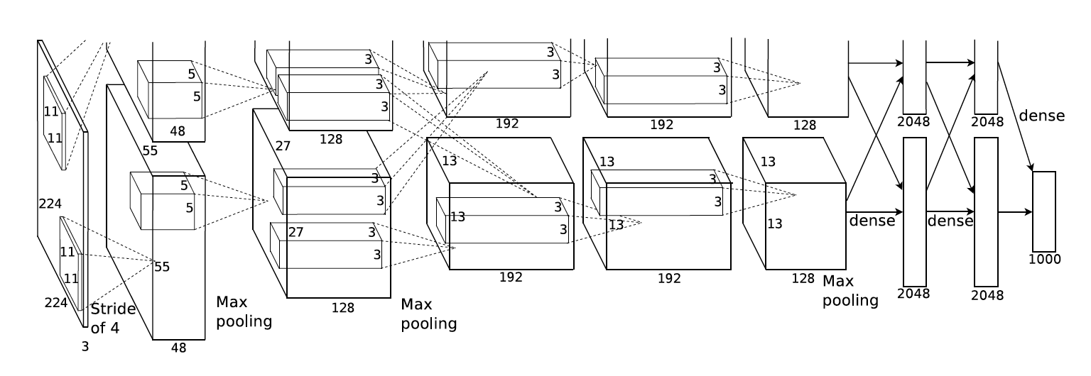
• 8 learned layers, 5 convolutional and 3 fully connected
• Based on some of Hinton's prior work, the ReLU function [f(x) = max(0,x)] was adopted as the activation function -- this non-saturating nonlinearity was much faster than saturating non-linearities like tanh and sigmoid. (Ref)

• The model was trained on multiple GPUs -- with half the neurons on each GPU. Certain kernel maps only took inputs from their own GPU, while some did across GPUs. This was decided via cross-validation. This scheme reduced top-1 and top-5 error rates by 1.7% and 1.2%, respectively as opposed to training a network of half the size on one GPU.

• The authors also mention that ReLUs have the desireable property that they don't require input normalisation to prevent them from saturating. However, it was found that normalisation did indeed reduce top-1 and top-5 error rates by 1.4% and 1.2%. They used a non-trainable layer that square-normalized the pixel values in a feature map within a local neighborhood. The normalisation occured across color channels

• Pooling layers in CNNs summarize the outputs of neighboring groups of neurons in the same kernel map. The authors chose to use overlapping pooling, which reduced the top-1 and top-5 error rates by 0.4% and 0.3%, respectively in comparison to the non-overlapping configuration.

Overall Architecture

• Maximizes the multinomial logistic regression objective, which is equivalent to maximizing the average across training cases of the log-probability of the correct label under the prediction distribution
• Trained using stochastic gradient descent with a batch size of 128 examples, momentum of 0.9, and weight decay of 0.0005

• Data Augmentation via the extraction of random 224x224 patches, and their horizontal reflections + altering the intensities of RGB channels (PCA on pixel values, and adding multiples of the principal components. e perform PCA on the set of RGB pixel values throughout the ImageNet training set. To each training image, we add multiples of the found principal components, with magnitues proportional to the corresponding eigenvalues times a random variable drawn from a Gaussian with mean zero and standard deviation 0.1. This scheme approximately captures an important property of natural images, namely, that object identity is invariant to changes in the intensity and color of the illumination. This scheme reduced the top-1 error rate by over 1%.

• Dropout, then recently introduced, consists of setting to zero the output of each hidden neuron with probability 0.5. The neurons which are “dropped out” in this way do not contribute to the forward pass and do not participate in back- propagation.
• At test time, we use all the neurons but multiply their outputs by 0.5, which is a reasonable approximation to taking the geometric mean of the predictive distributions produced by the exponentially-many dropout networks.

• Top-1 test set error of 37.5% on ILSVRC 2010
• Top-5 test set error rates of 17.0% on ILSVRC 2010
• Results show that a large, deep convolutional neural network is capable of achieving record- breaking results on a highly challenging dataset using purely supervised learning
• On the ILSVRC 2012 data, by averaging results over multiple CNNs, the authors were able to report the best performance of all the entries.

• The authors investigate the effect of the convolutional network depth on its accuracy in a large-scale image recognition setting.
• The primary objective was to improve on the work by Krizhevsky et al. (2012) and achieve better accuracy rates

• Their main contribution is a thorough evaluation of networks of increasing depth using an architecture with very small (3 × 3) convolution filters, which shows that a significant improvement on the prior-art configurations can be achieved by pushing the depth to 16–19 weight layers
• These findings were the basis of the authors' ImageNet Challenge 2014 submission, where our team secured the first and the second places in the localisation and classification tracks respectively

• During training, the input to the ConvNet is a 224x224 image (normalised by subtracting the mean per pixel)
• Image is passed through a stack of convolutional layers (with conv filters with a 3x3 receptive field) -- 1x1 receptive fields are also used at a point, which is essentially a linear transformation. The stride is 1 pixel
• Spatial pooling is performed via MaxPool (ref) layers, over 2x2 pixel windows with stride 2 -- this is after some of the conv layers, not all

• All the layers use a ReLU activation function
• None of the networks except for one used LRN, and the authors inferred that the use of LRN did not carry a specific benefit during training (contrary to what the folks over at UToronto figured out!)

• The authors demonstrate the benefits of smaller receptive fields, over the course of the larger number of layers - this incorporates more non-linear rectification layers making the decision function more discriminative, while also reducing the # of params
• The use of 1x1 conv filters created an increasingly non-linear decision function without affecting the receptive fields of the convolutional layers (the additional non-linearity is introduced by the ReLU)

• Very similar to the process followed by Krizhevsky, et all
• The batch size was set to 256, momentum to 0 .9. The training was regularised by weight decay, and the LR was dropped by a factor of 10 when the validation accuracy stopped improving.
• Learning was stopped after 370K iterations (74 epochs) -- the nets required less epochs to converge due to (a) implicit regularisation imposed by greater depth and smaller conv. filter sizes; (b) pre-initialisation of certain layers.
• The weights of the net weren't always randomly initialised. The shallowest net was first trained, and then those weights for those layers were used as starting points for the deeper nets

• Scaling was also utilised in order to manipulate image size
• Two approaches were considered: single-scale training with a fixed S, and multi-scale training, where S was selected from a range of [256, 512] -- this can be viewed as scale jittering, and was incorporated by fine-tuning a model trained on single-scale data

• The ConvNet architecture uses an interesting inference process -- involving the conversion of the net to a fully convolutional NN (referred to as dense evaluation)
• Upon inference, the FC layers are converted to convolutional layers, and the resulting fully convolutional net is used to optain a class-score map, with (# of channels = # of classes)
• Finally, to obtain a fixed-size vector of class scores for the image, the class score map is spatially averaged (sum-pooled: ref).
• Since the fully convolutional NN is applied to the whole image, there's no need to sample multiple crops -- the authors claim that this is far more efficient. However, they also point out that sampling multiple crops could lead to a performance gain

• The authors performed both single-scale, and multi-scale evaluation.
• For single scale evaluation (no scaling at test time), jittering at training time resulted in better results. This indicated that augmentation via jittering is indeed helpful for capturing certain image charecteristics across scales.

• Scale jittering at test time was also evaluated, and the results were found to be even better than those without jittering at test time
• This consists of running a model over several rescaled versions of a test image (corresponding to different values of Q), followed by averaging the resulting class posteriors.
• As before, the deepest configurations (D and E) performed the best, and scale jittering is better than training with a fixed smallest side S

• The authors evaluated very deep convolutional networks (up to 19 weight layers) for large- scale image classification.
• It was demonstrated that the representation depth is beneficial for the classification accuracy, and that state-of-the-art performance on the ImageNet challenge dataset can be achieved using a conventional ConvNet architecture (LeCun et al., 1989; Krizhevsky et al., 2012) with substantially increased depth.
• The authors also show (appendix) that our models generalise well to a wide range of tasks and datasets
• The results confirm the importance of depth in visual representations

• Achieves the new state of the art for classification and detection in ILSVRC 2014
• The authors increased the depth and width of the network while keeping the computational budget constant.
• 12x params as Krizhevsky et al, but with significantly better performance
• Introduces a new, efficient, deep neural architecture for vision: Inception

The Issues

• Max-pooling layers result in loss of accurate spatial information
• Increasing the number of layers is prone to overfitting + makes it difficult to propogate gradients
• Stacking large convolution operations is computationally expensive.

The Solution

• Can we use multiple, fixed, convolutional layers to capture more accurate spatial information, while also keeping everything computationally feasible?
• Inspired by a neuroscience model of the primate visual cortex -- can we use a series of fixed filters of different sizes to handle multiple scales
• We make the network wider instead

• Naive Inception Module: 3 different sizes of filters (1x1, 3x3, 5x5). Additionally, max pooling is also performed. The outputs are concatenated and sent to the next inception module.
• Dimensionality Reduced Module: A 1x1 convolution before the 3x3 and 5x5 convolutions, in order to limit the # of input channels (makes the operation cheaper)

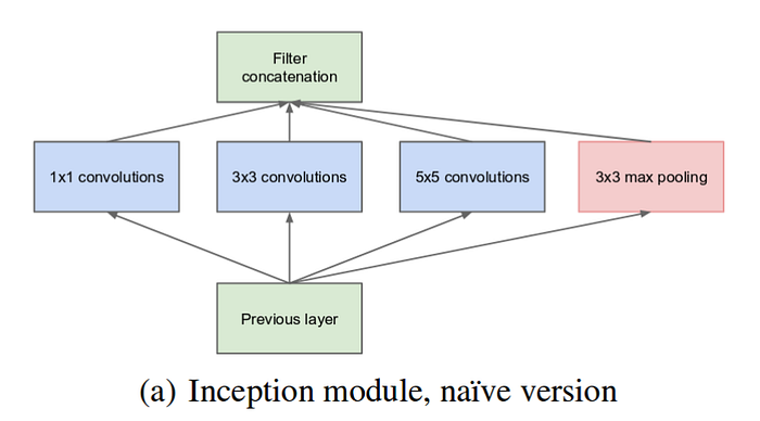
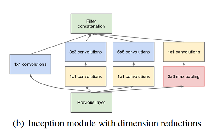
• All the convolutions, including those inside the Inception modules, use ReLU
• Input: 224×224 in the RGB color space with zero mean (normalise by mean)
• Note: "#3×3 reduce" and "#5×5 reduce" stands for the number of 1×1 filters in the reduction layer used before the 3×3 and 5×5 convolution

• The network is 22 layers deep when counting only layers with parameters (or 27 layers if we also count pooling)
• Average pooling is used before the final classification layer -- the authors found that average pooling (vs FC) improved the top-1 accuracy by about 0.6%, however the use of dropout remained essential even after removing the fully connected layers.

• Trained using the DistBelief distributed machine learning system using modest amount of model and data-parallelism
• Training used asynchronous stochastic gradient descent with 0.9 momentum and a fixed learning rate schedule (decreasing the learn- ing rate by 4% every 8 epochs).
• Data augmentation included sampling of various sized patches of the image whose size is distributed evenly between 8% and 100% of the image area with aspect ratio constrained to the interval [3/4,4/3]

• Emsembling, by training 7 GoogLeNet models -- models differed only in sampling and image order (and one model was a wider configuration)
• 144 crops per image were generated during testing, involving setting the image to 4 scales, obtaining the four corners, the center, and the original image resized as a square. The mirror images of all these images were also used

• The ILSVRC detection task is to produce bounding boxes around objects in images among 200 possible classes.
• Detected objects count as correct if they match the class of the groundtruth and their bounding boxes overlap by at least 50% (using the Jaccard index = [A intersection B) / (A union B]), with errors and false positives being penalised.
• GoogLeNet for detection is similar to the R-CNN by [6], but is augmented with the Inception model as the region classifier. Contrary to R-CNN though, bounding box regression was not used due to lack of time